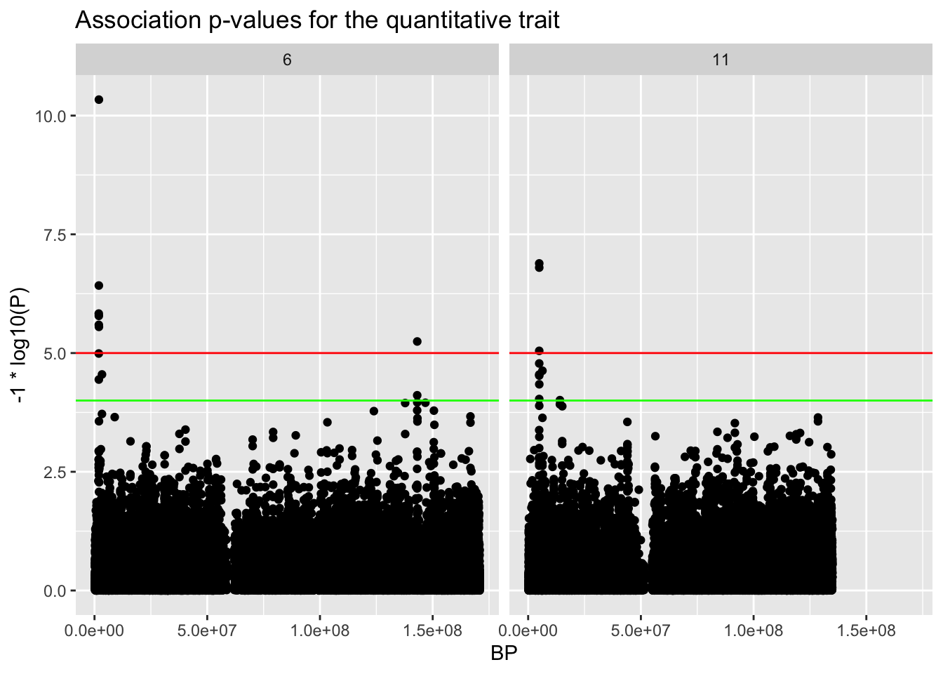
In an example genome-wide association scan, we had several hits:
library(tidyverse)library(knitr)library(pander)ASSOC.file <-"data/trait.qassoc.gz"b <-read_table(ASSOC.file)qplot(BP,-1.0*log10(P),main="Association p-values for the quantitative trait",data=b) +facet_wrap(~ CHR)+geom_hline(yintercept=5,col='red') +geom_hline(yintercept=4,col='green')
Here are our top hits:
top.hits <- b[order(b$P),c("CHR","BP","SNP","P")]row.names(top.hits) <-NULLpander(head(top.hits),caption="Top hits from our genome-wide association scan")
Top hits from our genome-wide association scan
CHR
BP
SNP
P
6
1942538
rs3800143
4.608e-11
11
4913057
rs10836914
1.295e-07
11
4913314
rs12577475
1.587e-07
6
1926650
rs11242725
3.785e-07
6
1880964
rs3800116
1.475e-06
6
1915129
rs3778552
1.646e-06
Now we’d like to annotate each of these SNPs in terms of nearby or overlapping genes.
While we could do this using online databases like UCSC Genome Browser (http://genome.ucsc.edu/cgi-bin/hgGateway), we could also use BioConductor R packages to write our own functions to retrieve this information into a nice tabular format, for each SNP, listing any gene that they might be in, including the SNP’s position and the gene boundaries.
29.1 Introductory Background
An Introduction to Bioconductor’s Packages for Working with Range Data
In “Bioinformatics Data Skills”, see Chapter 9 “Working with Range Data”
Bioinformatics Data Skills
Editor: Vince Buffalo
Publisher: O’Reilly
Web access: link
Hello Ranges: An Introduction to Analyzing Genomic Ranges in R. link
29.4 Install the needed Bioconductor libraries (one time only)
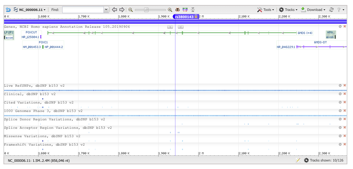
First, we need to figure out which genomic build was used in our data set. I usually do this by looking up the base pair positions of a couple of SNPs by hand in the ‘SNP’ data base. So if we go there and search for rs3800143, we end up on this web page:
GRangesList object of length 23459:
$`1`
GRanges object with 2 ranges and 2 metadata columns:
      seqnames            ranges strand |     tx_id     tx_name
         <Rle>         <IRanges>  <Rle> | <integer> <character>
  [1]    chr19 58858172-58864865      - |     70455  uc002qsd.4
  [2]    chr19 58859832-58874214      - |     70456  uc002qsf.2
  -------
  seqinfo: 93 sequences (1 circular) from hg19 genome

$`10`
GRanges object with 1 range and 2 metadata columns:
      seqnames            ranges strand |     tx_id     tx_name
         <Rle>         <IRanges>  <Rle> | <integer> <character>
  [1]     chr8 18248755-18258723      + |     31944  uc003wyw.1
  -------
  seqinfo: 93 sequences (1 circular) from hg19 genome

$`100`
GRanges object with 1 range and 2 metadata columns:
      seqnames            ranges strand |     tx_id     tx_name
         <Rle>         <IRanges>  <Rle> | <integer> <character>
  [1]    chr20 43248163-43280376      - |     72132  uc002xmj.3
  -------
  seqinfo: 93 sequences (1 circular) from hg19 genome

...
<23456 more elements>
The names of the list elements are Entrez gene IDs.
29.6 Construct a GRange containing our top SNP
Construct a GRange containing the top SNP. Note that the chromosome name needs to be in the same style as is seen in tx.by.gene. That is, the chromosome name needs to be “chr6” instead of ‘6’.
── Column specification ────────────────────────────────────────────────────────
cols(
  CHR = col_double(),
  SNP = col_character(),
  BP = col_double(),
  NMISS = col_double(),
  BETA = col_double(),
  SE = col_double(),
  R2 = col_double(),
  T = col_double(),
  P = col_double(),
  X10 = col_logical()
)
head(b)
# A tibble: 6 × 10
    CHR SNP           BP NMISS     BETA     SE         R2      T     P X10
  <dbl> <chr>      <dbl> <dbl>    <dbl>  <dbl>      <dbl>  <dbl> <dbl> <lgl>
1     6 rs9392298 203878  1573  0.110   0.0984 0.000801    1.12  0.262 NA
2     6 rs9405486 204072  1569  0.118   0.0982 0.000913    1.20  0.232 NA
3     6 rs7762550 204909  1574  0.0384  0.0685 0.000199    0.560 0.576 NA
4     6 rs1418706 205878  1575 -0.00783 0.0717 0.00000757 -0.109 0.913 NA
5     6 rs6920539 206528  1574  0.119   0.0955 0.000984    1.24  0.214 NA
6     6 rs9502959 206599  1575 -0.0317  0.0538 0.000220   -0.589 0.556 NA
Task: Using GRanges and associated Bioconductor tools, figure out if our top SNP, as ranked by the P-value (column P) from data frame b lies within an intron or exon.
For this, the functions exonsBy and intronsByTranscript might be useful.
Expand to see solution
29.10 Answer 1
The top SNP rs3800143 lies in an intron of GMDS (GDP-mannose 4,6-dehydratase), Gene ID: 2762.
From the output above, we find that our top SNP overlaps 2 sets of introns grouped by transcripts.
29.11 Question 2
While we have figure out above which gene our top SNP is in, what we worked out above involves very specific code. Now let’s try to generalize what we did above:
Task: Using GRanges and associated Bioconductor tools, write a function that takes as input a ranked list of the SNPS, and returns a nice table that lists the top N of these SNPs and any gene that they might be in, including the SNP position and the gene boundaries.
# snp.list = the ranked list of the top SNPs
# N = the number of top SNPs to annotate
snp.table <- function(snp.list, N=15) {

}
Apply your snp.table function to the top 15 SNPs in our example data set.
Hint
Use the subsetByOverlaps followed by the select(org.Hs.eg.db, ... approach described above in the Search for match and Convert Entrez Gene IDs to Gene Names sections above.
Expand to see solution
29.12 Answer 2
It is important to understand what the output of the findOverlaps function means.
Here, the ‘subjectHits’ is an index into top.snp and the queryHits is an index into gene.bounds.
So the first line indicates that the 13th SNP in top.snp overlaps the gene that is in the 3,269 slot of the gene.bounds object.
# snp.list = the ranked list of the top SNPs# N = the number of top SNPs to annotatesnp.table <-function(snp.list, N=15) {require(org.Hs.eg.db)require(TxDb.Hsapiens.UCSC.hg19.knownGene) txdb <- TxDb.Hsapiens.UCSC.hg19.knownGene tx.by.gene <-transcriptsBy(txdb, "gene")# Find the gene boundaries gene.bounds <-reduce(tx.by.gene)# Set up a GRange with the first N top SNPs top.snp <-with(snp.list[1:N, ], GRanges(seqnames =paste0("chr", CHR),IRanges(start = BP, width =1),SNP = SNP, P = P))# Find overlaps and hits top.snp.gene <-findOverlaps(gene.bounds, top.snp) hits <-subsetByOverlaps(gene.bounds, top.snp)# The SNP hits snp.info <-data.frame(SNP.ID =subjectHits(top.snp.gene),SNP.chr =seqnames(top.snp[subjectHits(top.snp.gene)]),ranges(top.snp[subjectHits(top.snp.gene)]),mcols(top.snp[subjectHits(top.snp.gene)]))# The Gene hits gene.info <-data.frame(gene.ID =queryHits(top.snp.gene),seqnames(gene.bounds[queryHits(top.snp.gene)]),ranges(gene.bounds[queryHits(top.snp.gene)]))# Reduce gene.info to distinct entries gene.info <- gene.info %>% dplyr::select(-group, -group.1) %>%distinct()# Construct a key linking SNPs to Genes key <-data.frame(gene.ID =queryHits(top.snp.gene),SNP.ID =subjectHits(top.snp.gene)) snp.gene <- key %>%left_join(gene.info, by ="gene.ID") %>%left_join(snp.info, by ="SNP.ID") gene.name <-select(org.Hs.eg.db, keys =names(hits),columns =c("ENTREZID", "SYMBOL", "GENENAME"), keytype ="ENTREZID") snp.gene <- snp.gene %>% dplyr::rename(ENTREZID = group_name) %>%left_join(gene.name, by ="ENTREZID") snp.gene <- snp.gene %>%arrange(P) snp.gene <-left_join(snp.list[1:N, ], snp.gene, by =c("SNP")) snp.gene <- snp.gene %>% dplyr::select(CHR, BP, SNP, P.x, SYMBOL, GENENAME, start.x, end.x, width.x) snp.gene <- snp.gene %>% dplyr::rename(P = P.x, start = start.x, end = end.x, width = width.x)return(snp.gene)}
(t <-snp.table(top.hits, 15)) %>%kable(digits=15)
Warning in .local(x, row.names, optional, ...): 'optional' argument was ignored
'select()' returned 1:1 mapping between keys and columns
CHR
BP
SNP
P
SYMBOL
GENENAME
start
end
width
6
1942538
rs3800143
4.608e-11
GMDS
GDP-mannose 4,6-dehydratase
1624035
2245868
621834
11
4913057
rs10836914
1.295e-07
NA
NA
NA
NA
NA
11
4913314
rs12577475
1.587e-07
NA
NA
NA
NA
NA
6
1926650
rs11242725
3.785e-07
GMDS
GDP-mannose 4,6-dehydratase
1624035
2245868
621834
6
1880964
rs3800116
1.475e-06
GMDS
GDP-mannose 4,6-dehydratase
1624035
2245868
621834
6
1915129
rs3778552
1.646e-06
GMDS
GDP-mannose 4,6-dehydratase
1624035
2245868
621834
6
1908210
rs2875711
2.550e-06
GMDS
GDP-mannose 4,6-dehydratase
1624035
2245868
621834
6
1955398
rs9378664
2.809e-06
GMDS
GDP-mannose 4,6-dehydratase
1624035
2245868
621834
6
143144885
rs926372
5.704e-06
HIVEP2
HIVEP zinc finger 2
143072604
143266338
193735
11
4912192
rs10836912
8.977e-06
NA
NA
NA
NA
NA
6
1899671
rs3800122
1.022e-05
GMDS
GDP-mannose 4,6-dehydratase
1624035
2245868
621834
11
4910224
rs2570591
1.656e-05
NA
NA
NA
NA
NA
11
6340706
rs1051992
2.356e-05
CAVIN3
caveolae associated protein 3
6340176
6341740
1565
6
3317016
rs4959804
2.821e-05
SLC22A23
solute carrier family 22 member 23
3269207
3456793
187587
11
4915072
rs1816448
2.834e-05
NA
NA
NA
NA
NA
dim(t)
[1] 15 9
Here’s an alternate way to construct the SNP table which is an incomplete example because it doesn’t include the gene boundaries. However, it is simpler than the function above because it avoids the construction of a key and the left_joins used above by looping through each SNP, one by one:
'select()' returned 1:1 mapping between keys and columns
'select()' returned 1:1 mapping between keys and columns
'select()' returned 1:1 mapping between keys and columns
'select()' returned 1:1 mapping between keys and columns
'select()' returned 1:1 mapping between keys and columns
'select()' returned 1:1 mapping between keys and columns
'select()' returned 1:1 mapping between keys and columns
'select()' returned 1:1 mapping between keys and columns
'select()' returned 1:1 mapping between keys and columns
'select()' returned 1:1 mapping between keys and columns
CHR
BP
SNP
P
Symbol
Gene name
6
1942538
rs3800143
4.608e-11
GMDS
GDP-mannose 4,6-dehydratase
11
4913057
rs10836914
1.295e-07
NA
NA
11
4913314
rs12577475
1.587e-07
NA
NA
6
1926650
rs11242725
3.785e-07
GMDS
GDP-mannose 4,6-dehydratase
6
1880964
rs3800116
1.475e-06
GMDS
GDP-mannose 4,6-dehydratase
6
1915129
rs3778552
1.646e-06
GMDS
GDP-mannose 4,6-dehydratase
6
1908210
rs2875711
2.550e-06
GMDS
GDP-mannose 4,6-dehydratase
6
1955398
rs9378664
2.809e-06
GMDS
GDP-mannose 4,6-dehydratase
6
143144885
rs926372
5.704e-06
HIVEP2
HIVEP zinc finger 2
11
4912192
rs10836912
8.977e-06
NA
NA
6
1899671
rs3800122
1.022e-05
GMDS
GDP-mannose 4,6-dehydratase
11
4910224
rs2570591
1.656e-05
NA
NA
11
6340706
rs1051992
2.356e-05
CAVIN3
caveolae associated protein 3
6
3317016
rs4959804
2.821e-05
SLC22A23
solute carrier family 22 member 23
11
4915072
rs1816448
2.834e-05
NA
NA
dim(t)
[1] 15 6
29.13 Question 3
Task: Using GRanges and associated Bioconductor tools, write a function that takes as input a ranked list of the SNPS, and returns a nice table that lists the top N of these SNPs and the closest flanking genes on both sides, including the SNP position and the gene boundaries.
# snp.list = the ranked list of the top SNPs
# N = the number of top SNPs to annotate
snp.flank <- function(snp.list, N=15) {

}
Apply your snp.flank function to the top 15 SNPs in our example data set.
Note that the purpose here is to think more about how to creatively use GRanges than to search for nice annotation packages.
Hint
The GenomicRanges package has a useful function nearest that can be used to find the nearest gene.
Note that if we want to augment information about the nearest gene with the genes that precede and follow each top SNP, we could use functions like this:
Note that we need to set up the txdb object within the function itself to avoid creating a dependence on the global txdb object. Although, it might be more efficient to create the txdb object once and pass it in via a function parameter instead of recreating it each time the function is called.
Here we use require statements to indicate dependence on certain libraries having been loaded, but if this were part of an R package, we’d take care of library dependencies at the package level instead of inside of specific functions. Usually when writing functions, we assume that all of the required packages have been loaded, so we tend not to use the library or the require command within functions.
# snp.list = the ranked list of the top SNPs# N = the number of top SNPs to annotatesnp.flank <-function(snp.list, N=15) {require(org.Hs.eg.db)require(TxDb.Hsapiens.UCSC.hg19.knownGene) txdb <- TxDb.Hsapiens.UCSC.hg19.knownGene tx.by.gene <-transcriptsBy(txdb, "gene")# Find the gene boundaries gene.bounds <-reduce(tx.by.gene)# Set up a GRange with the first N top SNPs top.snp <-with(snp.list[1:N, ], GRanges(seqnames =paste0("chr", CHR),IRanges(start = BP, width =1),SNP = SNP, P = P))# Find overlaps and hits top.snp.gene <-findOverlaps(gene.bounds, top.snp) hits <-subsetByOverlaps(gene.bounds, top.snp)# The SNP hits snp.info <-data.frame(SNP.ID =subjectHits(top.snp.gene),SNP.chr =seqnames(top.snp[subjectHits(top.snp.gene)]),ranges(top.snp[subjectHits(top.snp.gene)]),mcols(top.snp[subjectHits(top.snp.gene)]))# The Gene hits gene.info <-data.frame(gene.ID =queryHits(top.snp.gene),seqnames(gene.bounds[queryHits(top.snp.gene)]),ranges(gene.bounds[queryHits(top.snp.gene)]))# Reduce gene.info to distinct entries gene.info <- gene.info %>% dplyr::select(-group, -group.1) %>%distinct()# Construct a key linking SNPs to Genes key <-data.frame(gene.ID =queryHits(top.snp.gene),SNP.ID =subjectHits(top.snp.gene)) snp.gene <- key %>%left_join(gene.info, by ="gene.ID") %>%left_join(snp.info, by ="SNP.ID") gene.name <-select(org.Hs.eg.db, keys =names(hits),columns =c("ENTREZID", "SYMBOL", "GENENAME"), keytype ="ENTREZID") snp.gene <- snp.gene %>% dplyr::rename(ENTREZID = group_name) %>%left_join(gene.name, by ="ENTREZID") snp.gene <- snp.gene %>%arrange(P) snp.gene <-left_join(snp.list[1:N, ], snp.gene, by =c("SNP")) snp.gene <- snp.gene %>% dplyr::select(CHR, BP, SNP, P.x, SYMBOL, GENENAME, start.x, end.x, width.x) snp.gene <- snp.gene %>% dplyr::rename(P = P.x, start = start.x, end = end.x, width = width.x)# Now find the nearest genes genes <-genes(txdb, columns ="gene_id")# Find the Nearest gene nearest_gene_index <-nearest(top.snp, genes) EntrezID <-unlist(genes[nearest_gene_index]$gene_id) lookup <-select(org.Hs.eg.db, keys = EntrezID, keytype ="ENTREZID",columns =c("SYMBOL", "GENENAME")) symbol <- lookup$SYMBOL genename <- lookup$GENENAME nearest <-bind_cols(SNP =mcols(top.snp)$SNP, EntrezID = EntrezID,symbol = symbol, genename = genename,start =unlist(start(gene.bounds[EntrezID, ])),end =unlist(end(gene.bounds[EntrezID, ])))if (all.equal(mcols(top.snp)$SNP, nearest$SNP)) { snp.gene$Nearest <- nearest$symbol snp.gene$N.GENENAME <- nearest$genename snp.gene$N.start <- nearest$start snp.gene$N.end <- nearest$end }# Find the preceding genes precede_gene_index <-precede(top.snp, genes) EntrezID <-unlist(genes[precede_gene_index]$gene_id) lookup <-select(org.Hs.eg.db, keys = EntrezID, keytype ="ENTREZID",columns =c("SYMBOL", "GENENAME")) symbol <- lookup$SYMBOL genename <- lookup$GENENAME precede <-bind_cols(SNP =mcols(top.snp)$SNP, EntrezID = EntrezID,symbol = symbol, genename = genename,start =unlist(start(gene.bounds[EntrezID, ])),end =unlist(end(gene.bounds[EntrezID, ])))if (all.equal(mcols(top.snp)$SNP, precede$SNP)) { snp.gene$Precede <- precede$symbol snp.gene$P.GENENAME <- precede$genename snp.gene$P.start <- precede$start snp.gene$P.end <- precede$end }# Find the following genes follow_gene_index <-follow(top.snp, genes) EntrezID <-unlist(genes[follow_gene_index]$gene_id) lookup <-select(org.Hs.eg.db, keys = EntrezID, keytype ="ENTREZID",columns =c("SYMBOL", "GENENAME")) symbol <- lookup$SYMBOL genename <- lookup$GENENAME follow <-bind_cols(SNP =mcols(top.snp)$SNP, EntrezID = EntrezID,symbol = symbol, genename = genename,start =unlist(start(gene.bounds[EntrezID, ])),end =unlist(end(gene.bounds[EntrezID, ])))if (all.equal(mcols(top.snp)$SNP, follow$SNP)) { snp.gene$Follow <- follow$symbol snp.gene$F.GENENAME <- follow$genename snp.gene$F.start <- follow$start snp.gene$F.end <- follow$end }return(snp.gene)}
(t <-snp.flank(top.hits, 15)) %>%kable(digits=15)
Warning in .local(x, row.names, optional, ...): 'optional' argument was ignored
'select()' returned 1:1 mapping between keys and columns
  403 genes were dropped because they have exons located on both strands of the
  same reference sequence or on more than one reference sequence, so cannot be
  represented by a single genomic range.
  Use 'single.strand.genes.only=FALSE' to get all the genes in a GRangesList
  object, or use suppressMessages() to suppress this message.
'select()' returned many:1 mapping between keys and columns
'select()' returned many:1 mapping between keys and columns
'select()' returned many:1 mapping between keys and columns
 Does our top SNP overlap any exons?