23 R Recoding Reshaping Exercise
23.1 Key points
Here are some key points regarding recoding and reshaping data in R:
- Count the number of times
ID2is duplicatedsum(duplicated(b$ID2))
- List all rows with a duplicated
c1valuef %>% group_by(c1) %>% filter(n()>1)
- Recode data using
left_join - Pivot data from long to wide
pivot_wider
- Pivot data from wide to long
pivot_longer
- Useful table commands
table()addmargins(table())prop.table(table(), margin)
23.2 Download example data
23.3 Recoding data
Different parts of the data may have different ID systems
Clinical ID
Laboratory ID
Genotyping service ID
Need a dictionary or key to translate one type of key into another key
23.4 A dictionary
- A dictionary defines a one-to-one correspondence between keys and values
- keys must be unique
23.5 Recoding data
Good practice to output old IDs as well as new IDs into the output files
Permits checking
Have to convey results back to your collaborators using their ID system
Suppose we have been given these data:
    ==> study2_ped.txt <==
    ID1     sex     aff2
    1       M       1
    2       M       2
    ==> study2_pheno.txt <==
    ID2     sex     t
    E544    M       3.34263153909733
    E853    M       5.35786611210859
    ==> study2_snp.txt <==
    ID2     SNPID2          all1    all2
    E544    Aff-S-3212091   A       T
    E853    Aff-S-1032132   A       A
The clinicians used an integer for the Person IDs:
    ==> study2_ped.txt <==
    ID1     sex     aff2
    1       M       1
    2       M       2
The serum assay laboratory used a different set of Person IDs starting with the letter ’E’:
    ==> study2_pheno.txt <==
    ID2     sex     t
    E544    M       3.34263153909733
    E853    M       5.35786611210859
While the genotyping lab also used ’E’ Person IDs, they did not use ’rs’ SNP IDs:
    ==> study2_snp.txt <==
    ID2     SNPID2          all1    all2
    E544    Aff-S-3212091   A       T
    E853    Aff-S-1032132   A       A
Keys
- To use these data together, we need to translate Person IDs and SNP IDs so that all of our files are using the same IDs (e.g. so they all speak the same language).
- To do this, we need translation keys:
==> study2_key1.txt <==
ID1     ID2
1       E544
2       E853

==> study2_key2.txt <==
rsID    SNPID2
rs35814900      Aff-S-3212091
rs28370510      Aff-S-1032132
23.6 Duplicates
Note above that we said that the keys must be unique.
Question: How would you check in R that the keys are unique? For example, how would you check for duplicates in the ID2 column of ‘study2_key1.txt’?
Answer: In R, the duplicated function can be used to check for duplicates
23.6.1 Counting duplicates
To count the number of duplicated ID’s, we can take advantage of the fact that a TRUE value behaves as a 1 and a FALSE value behaves as a 0 when a logicial variable is used in a numeric computation.
23.6.2 Checking for duplicates
How do we return every row that contains a duplicate?
Another way to list all of the rows containing a duplicated ‘c1’ value:
Yet another way to list all of the rows containing a duplicated ‘c1’ value using functions from the ‘tidyverse’ package:
23.6.3 Key points: Duplicates
Here are some key points regarding detecting duplicates:
- Count the number of times
ID2is duplicatedsum(duplicated(b$ID2))
- List all rows with a duplicated
c1valuef %>% group_by(c1) %>% filter(n()>1)
23.7 Project 1 Data
In the ds data frame we have the synthetic yet realistic data we will be using in Project 1.
In the dd data frame we have the corresponding data dictionary.
23.8 Exercise 1: duplicated values
Skill: Checking for duplicated IDs
Using the ds data frame from Project 1, check if there are any duplicated sample_id’s using the duplicated command. If so, count how many duplicated sample_id’s there are.
Construct a table of the number of times each sample_id is duplicated:
Note that it is important to be aware of missing IDs. So when constructing tables of counts using the table command, the useNA argument controls if the table includes counts of NA values.
How many sample_id’s are NA’s?
Check if there are any duplicated subject_ids
We can check if there are any duplicated subject_id’s by counting how many duplicates there are.
23.9 Checking for duplicates
How do we return every row that contains a duplicate?
This approach only does not return every row that contains a duplicated ID:
23.10 Counting the number of occurences of the ID
23.11 Count sample_id duplicates
Using Tidyverse commands, count how many times each sample_id occcurs in the ds data frame, reporting the counts in descending order, from highest to lowest.
23.12 Checking for duplicates
Here we list all of the rows containing a duplicated ‘ID’ value using functions from the ‘tidyverse’ package:
23.12.1 How to list all duplicates
Use Tidyverse commands to list (1) all duplicates for sample_id and (2) all duplicates for subject_id. Sort the results by the ID.
23.12.2 Sample ID
23.12.3 Subject ID
23.13 Reshaping data
23.13.1 Download example data
23.13.2 Long & wide PLINK data
For large-scale data, PLINK is very useful for converting from ‘long’ to ‘wide’
Long: ped, per, rsID, allele 1, allele 2
Wide: ped, per, SNP1 allele 1, SNP1 allele 2, SNP2 allele 1, SNP2 allele 2, …
CAUTION: When reading long data, PLINK does not warn about multiple genotypes for the same person, but rather uses the final one read in.
Long format data: one row per genotype
23.13.3 reshape
So here we have two SNPs typed per person, and we want to convert from ’long’ format to ’wide’ format:
Wide format data: one row per individual
Check that it worked correctly:
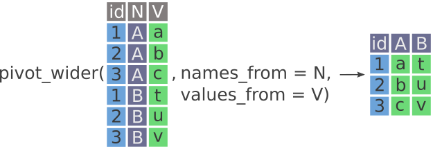
23.13.4 pivot_wider
Here’s a nice illustration from “Intermediate Reproducible Research in R” (which they shared under a CC_BY 4.0 license), where they caption this figure as follows:
“Pivot wider in tidyr, where a set of stacked”groups” in the data on the left are placed side-by-side as new columns in the output data on the right. Notice how the values in the column N, which is used in the names_from argument, are used as the names for the new columns A and B in the new data.”
For more detail, see
https://r-cubed-intermediate.rostools.org/sessions/pivots
Using pivot_wider from tidyverse:
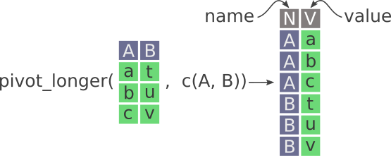
23.13.5 pivot_longer
Here’s a nice illustration from “Intermediate Reproducible Research in R” (which they shared under a CC_BY 4.0 license), where they caption this figure as follows:
“Pivot longer in tidyr. New columns are called name and value. Notice how the values in A and B columns are stacked on top of each other in the newly created V column.”
For more detail, see
23.13.6 Key points
Here are some key points regarding reshaping data in R:
- Pivot data from long to wide
pivot_wider
- Pivot data from wide to long
pivot_longer
23.14 Exercise 2: Reshaping data
Skill: Reshaping data
Select only three columns “sample_id”, “Sample_trimester”, “Gestationalage_sample” from the ds data frame, and then reshape from ‘long’ format to ‘wide’ format using pivot_wider, taking time as the “Sample_trimester”.
23.14.1 Comment
View b2 via the View(b2) command in RStudio - it nicely put all the different gestational age observations into one list for each sample_id x Sample_trimester combination.
23.15 Exercise 3: Aggregating data
Skill: Aggregating data
Make a table showing the proportion of blacks and whites that are controls and cases.
Construct more readable tables with labels using xtabs
23.15.2 xtabs table with labels
Create a count cross table using Tidyverse commands
Or we can do this with pivot_wider instead as follows:
Create a proportion cross table using Tidyverse commands
23.16 Exercise 4: Summarizing within groups
The split command
split(x,f): divides the data x into the groups defined by f, where f is a factor or list of factors.
To illustrate this, we split ds into a list of data frames by baby_sex while only keeping the baby_sex and race columns:
Commands from the apply family
We can then apply a function to each element of the list using lapply or sapply:
The lapply(X, FUN) lapply returns a list of the same length as X, each element of which is the result of applying FUN to the corresponding element of X.
The sapply(X, FUN) function is a user-friendly version of lapply by default returning a vector, matrix or array if appropriate.
Skill: Summarizing within groups
Use the split/sapply approach to apply the summary command to the “Gestationalage_sample” within each “Sample_trimester” group.
Note: With split(x, f), any missing values in the factor f are dropped together with the corresponding values of x.
23.17 Recoding data
23.17.1 Recoding data using look-up tables
Approach 1
- Implement our dictionaries using look-up tables
- Use a named vector.
Here’s an example of how to do this:
- Use the information in
study2_key1.txtto set up a dictionarydictPerthat maps ‘E’ person IDs to integer person IDs.
- Read in study2_pheno.txt, and using
dictPer, translate the person IDs and write it out again with the translated person IDs.
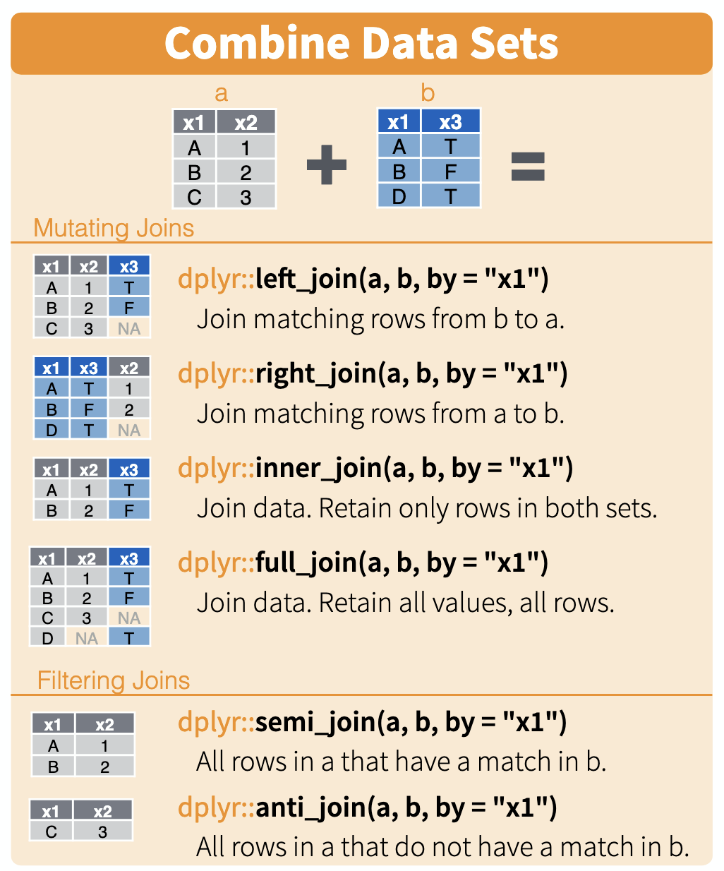
23.17.2 Recoding data using left joins
Joins illustrated
Here is a nice illustration of joins from RStudio (which they shared under a CC_BY 4.0 license)
Approach 2
- Implement our dictionaries using left joins
Here’s an example of how to do this:
- Read in study2_pheno.txt, and using
dictPer, translate the person IDs and write it out again with the translated person IDs.
23.18 Exercise 5: Recoding data
Approach 1
- Implement our dictionaries using look-up tables
- Use a named vector.
Skill:: Recoding IDs using a dictionary
Create a new subject ID column named “subjectID” where you have used the DictPer named vector to recode the original “subject_id” IDs into integer IDs.
Note: If the DictPer named vector is not available, be sure to load the Project 1 data above using the commands in the ‘Project 1 Data’ section.
Approach 2
- Implement our dictionaries using left joins
23.18.1 Comment
I usually prefer to use a merge command like left_join to merge in the new IDs into my data frame.
23.19 Exercise 6: Filtering rows
Skill: Filtering rows.
Create a data frame tri1 containing the records for Trimester 1, and a second data frame tri2 containing the records for Trimester 2.
23.20 Exercise 7: Selecting columns
Skill: Selecting columns
Update tri1 and tri2 to only contain the three columns “sample_id”, “Sample_trimester”, “Gestationalage_sample”
23.15.1 Comment:
The
marginparameter of theprop.tablecommand has to be specified in order to get the desired answer: “1 indicates rows, 2 indicates columns.